Python pytrends Line Chart Tutorial

Let’s do a Python pytrends Tutorial! The pytrends library is the unofficial API for Google Trends. Google Trends is a research tool that is used to find out what keywords are trending in Google Search.

First we have to install it, which we can do with the following code: pip install pytrends . This library requires Python 3.3+ to work, so make sure you have a suitable version. We will be using Python 3.8.10 for this example.

Next, let’s write some code:

from pytrends.request import TrendReq
import pandas as pd

pytrends = TrendReq(hl='en-US', tz=400)

kw_list = ["dating"]

dating_trends_1mo  = pytrends.get_historical_interest(kw_list, year_start=2022, month_start=1, day_start=1, hour_start=0, year_end=2022, month_end=2, day_end=1, hour_end=0, cat=0, geo='US-CA', gprop='', sleep=60)

dating_trends_1mo.to_csv("dating_trends_1mo.csv")

Let’s explain what is happening here:

1. We import the pytrends.request library and the TrendReq method. We also import the pandas library because the result of our request will be a dataframe which we will then export as a CSV file.
2. Method TrendReq() is our pytrends request. We supply two parameters: hl with value en-US which is the host language for accessing Google Trends and tz which is the timezone offset for our current location. The timezone is important so that we get the correct time and date in our result.
3. List kw_list is a list of our keywords for which we would like to retrieve Google Trends data. In this case we want to find out the trend for topic keyword dating.😍
4. The pytrends.get_historical_interest() method will give us the historical hourly interest for the given keyword according to Google data as a dataframe, which we will store as dating_trends_1mo. We supply the start date time and end date time, obviously. We want data for the month of January 2022. Additionally, we supply the following parameters:
   • cat is 0 which will reference all Google Trends categories
   • geo is the location. We want to retrieve hourly interest for California, USA
   • gprop is the Google Property to use, by default this is web search
   • sleep spaces our API calls so that we aren’t rate limited
5. We save our results to a CSV file on disk. The file will reside in the same folder as our python script.

When the above code executes, we should have a new file on disk called: dating_trends_1mo.csv. It will have hourly interest for the topic of Dating for the state of California, USA for January 2022. The “interest” is rated on the scale of 1 to 100. Rating 100 means high interest.

We can take our example a step further and produce a line chart that will give is a visual of the trend. First, make sure Plotly is installed. If not, the command is pip install plotly-express.

Here is the code:

import pandas as pd
import plotly.express as px

df = pd.read_csv('dating_trends_1mo.csv')

df['date'] = pd.to_datetime(df['date'], errors='coerce')

fig = px.line(df.groupby(df.date.dt.day).agg({'dating':'mean'}), \
                y = 'dating', \
                title='Pytrends for Keyword DATING January 2022')
fig.show()

Let’s explain what is happening here:

1. We import our plotly library and pandas as usual.
2. We read our previously generated CSV file from disk: dating_trends_1mo.csv
3. We ensure that the date column is a proper date.
4. We group the date column by day and find the average rating per day. This makes our graph cleaner.
5. We create a line graph that shows the pytrends data visually.

When the code executes, you should see the following graph on the screen:

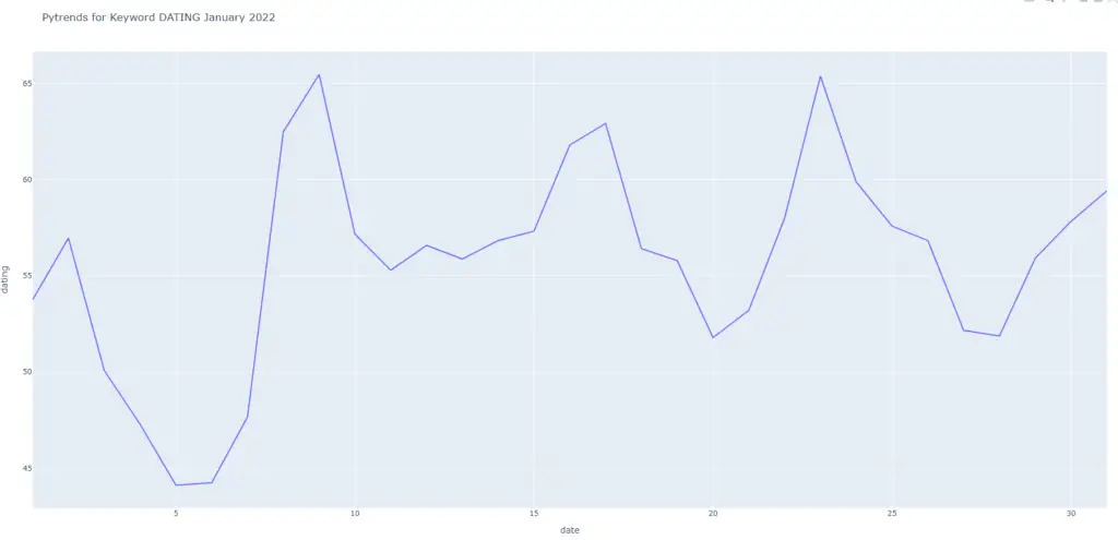
Easy right? Now we see the average day-to-day pytrends data for Jan 2022 for California, USA. Visuals are always a good idea when you are talking about any type of trend data. Below is our full code:

from pytrends.request import TrendReq

import pandas as pd
import plotly.express as px


pytrends = TrendReq(hl='en-US', tz=400)

kw_list = ["dating"]

dating_trends_1mo  = pytrends.get_historical_interest(kw_list, year_start=2022, month_start=1, day_start=1, hour_start=0, year_end=2022, month_end=2, day_end=1, hour_end=0, cat=0, geo='US-CA', gprop='', sleep=60)
dating_trends_1mo.to_csv("dating_trends_1mo.csv")

df = pd.read_csv('dating_trends_1mo.csv')
df['date'] = pd.to_datetime(df['date'], errors='coerce')

fig = px.line(df.groupby(df.date.dt.day).agg({'dating':'mean'}), \
                y = 'dating', \
                title='Pytrends for Keyword DATING January 2022')
fig.show()

Find pytrends on Github HERE. Thanks for reading and good luck! 👌👌👌